
Process Macro Model 14, 15 해석 관련 질문
교수님, 안녕하십니까. 현재 석사 4학차 재학중인 대학원생입니다.
유튜브를 통해 교수님을 알게 되었고, 논문 작성 및 해석에 막힘이 있어 이렇게 글을 남깁니다.
Process Macro 1번 모델로 X → Y에서 W의 조절효과, M → Y에서 W의 조절효과를 확인하였고 모두 유의하다고 나왔습니다.
또한 4번 모델 X → M → Y의 매개효과도 유의하였습니다.
그러면 Process Macro 14번 모델보다 15번 모델에 적합할 것으로 생각하여, 통계를 돌려보았지만
14번 모델의 M*W → Y의 조절된 매개효과가 유의하다고 나오지만, 15번 모델에선 M*W → Y가 유의하지 않고, X*W → Y가 유의한 것으로 나와 혼란을 겪고 있습니다.
질문은 이상입니다.
Model 14와 15의 통계 결과는 아래 첨부하겠습니다.
Run MATRIX procedure:
***************** PROCESS Procedure for SPSS Version 4.2 *****************
Written by Andrew F. Hayes, Ph.D. www.afhayes.com
Documentation available in Hayes (2022). www.guilford.com/p/hayes3
**************************************************************************
Model : 14
Y : dep_avg
X : jss_avg
M : scri_avg
W : scom_avg
Sample
Size: 334
**************************************************************************
OUTCOME VARIABLE:
scri_avg
Model Summary
R R-sq MSE F df1 df2 p
.5163 .2666 .4569 120.6723 1.0000 332.0000 .0000
Model
coeff se t p LLCI ULCI
constant -1.7564 .1641 -10.7025 .0000 -2.0793 -1.4336
jss_avg .6500 .0592 10.9851 .0000 .5336 .7664
**************************************************************************
OUTCOME VARIABLE:
dep_avg
Model Summary
R R-sq MSE F df1 df2 p
.8310 .6905 .1166 183.4891 4.0000 329.0000 .0000
Model
coeff se t p LLCI ULCI
constant 1.2983 .1017 12.7667 .0000 1.0983 1.4984
jss_avg .2307 .0357 6.4647 .0000 .1605 .3009
scri_avg .4359 .0415 10.5098 .0000 .3543 .5175
scom_avg -.1698 .0526 -3.2294 .0014 -.2732 -.0664
Int_1 -.1579 .0357 -4.4237 .0000 -.2281 -.0877
Product terms key:
Int_1 : scri_avg x scom_avg
Test(s) of highest order unconditional interaction(s):
R2-chng F df1 df2 p
M*W .0184 19.5690 1.0000 329.0000 .0000
----------
Focal predict: scri_avg (M)
Mod var: scom_avg (W)
Conditional effects of the focal predictor at values of the moderator(s):
scom_avg Effect se t p LLCI ULCI
-.5851 .5283 .0466 11.3484 .0000 .4367 .6199
.0000 .4359 .0415 10.5098 .0000 .3543 .5175
.5851 .3436 .0463 7.4167 .0000 .2524 .4347
There are no statistical significance transition points within the observed
range of the moderator found using the Johnson-Neyman method.
Conditional effect of focal predictor at values of the moderator:
scom_avg Effect se t p LLCI ULCI
-1.6046 .6892 .0709 9.7196 .0000 .5497 .8287
-1.4471 .6644 .0664 10.0004 .0000 .5337 .7950
-1.2895 .6395 .0621 10.2909 .0000 .5172 .7617
-1.1320 .6146 .0581 10.5829 .0000 .5004 .7289
-.9745 .5898 .0543 10.8629 .0000 .4830 .6966
-.8170 .5649 .0508 11.1099 .0000 .4649 .6649
-.6595 .5400 .0478 11.2941 .0000 .4460 .6341
-.5020 .5152 .0453 11.3768 .0000 .4261 .6042
-.3445 .4903 .0433 11.3146 .0000 .4051 .5756
-.1870 .4654 .0421 11.0683 .0000 .3827 .5482
-.0295 .4406 .0415 10.6169 .0000 .3589 .5222
.1280 .4157 .0417 9.9689 .0000 .3337 .4977
.2855 .3909 .0427 9.1641 .0000 .3069 .4748
.4431 .3660 .0443 8.2619 .0000 .2788 .4531
.6006 .3411 .0466 7.3250 .0000 .2495 .4327
.7581 .3163 .0494 6.4046 .0000 .2191 .4134
.9156 .2914 .0526 5.5354 .0000 .1878 .3950
1.0731 .2665 .0563 4.7360 .0000 .1558 .3772
1.2306 .2417 .0602 4.0131 .0001 .1232 .3601
1.3881 .2168 .0644 3.3660 .0009 .0901 .3435
1.5456 .1919 .0688 2.7896 .0056 .0566 .3273
1.7031 .1671 .0734 2.2772 .0234 .0227 .3114
Data for visualizing the conditional effect of the focal predictor:
Paste text below into a SPSS syntax window and execute to produce plot.
DATA LIST FREE/
scri_avg scom_avg dep_avg .
BEGIN DATA.
-.7881 -.5851 1.6047
.0000 -.5851 2.0211
.7881 -.5851 2.4374
-.7881 .0000 1.5782
.0000 .0000 1.9217
.7881 .0000 2.2653
-.7881 .5851 1.5516
.0000 .5851 1.8224
.7881 .5851 2.0932
END DATA.
GRAPH/SCATTERPLOT=
scri_avg WITH dep_avg BY scom_avg .
****************** DIRECT AND INDIRECT EFFECTS OF X ON Y *****************
Direct effect of X on Y
Effect se t p LLCI ULCI
.2307 .0357 6.4647 .0000 .1605 .3009
Conditional indirect effects of X on Y:
INDIRECT EFFECT:
jss_avg -> scri_avg -> dep_avg
scom_avg Effect BootSE BootLLCI BootULCI
-.5851 .3434 .0392 .2693 .4238
.0000 .2834 .0338 .2202 .3525
.5851 .2233 .0331 .1600 .2904
Index of moderated mediation:
Index BootSE BootLLCI BootULCI
scom_avg -.1026 .0223 -.1471 -.0590
*********************** ANALYSIS NOTES AND ERRORS ************************
Level of confidence for all confidence intervals in output:
95.0000
Number of bootstrap samples for percentile bootstrap confidence intervals:
10000
W values in conditional tables are the mean and +/- SD from the mean.
NOTE: The following variables were mean centered prior to analysis:
scom_avg scri_avg
------ END MATRIX -----
아래는 15번 모델입니다.
Run MATRIX procedure:
***************** PROCESS Procedure for SPSS Version 4.2 *****************
Written by Andrew F. Hayes, Ph.D. www.afhayes.com
Documentation available in Hayes (2022). www.guilford.com/p/hayes3
**************************************************************************
Model : 15
Y : dep_avg
X : jss_avg
M : scri_avg
W : scom_avg
Sample
Size: 334
**************************************************************************
OUTCOME VARIABLE:
scri_avg
Model Summary
R R-sq MSE F df1 df2 p
.5163 .2666 .4569 120.6723 1.0000 332.0000 .0000
Model
coeff se t p LLCI ULCI
constant .0000 .0370 .0000 1.0000 -.0728 .0728
jss_avg .6500 .0592 10.9851 .0000 .5336 .7664
**************************************************************************
OUTCOME VARIABLE:
dep_avg
Model Summary
R R-sq MSE F df1 df2 p
.8349 .6970 .1145 150.8903 5.0000 328.0000 .0000
Model
coeff se t p LLCI ULCI
constant 1.9240 .0226 85.1972 .0000 1.8795 1.9684
jss_avg .2119 .0361 5.8729 .0000 .1409 .2828
scri_avg .4312 .0411 10.4823 .0000 .3503 .5122
scom_avg -.2176 .0551 -3.9469 .0001 -.3260 -.1091
Int_1 -.1700 .0641 -2.6522 .0084 -.2962 -.0439
Int_2 -.0812 .0457 -1.7785 .0763 -.1711 .0086
Product terms key:
Int_1 : jss_avg x scom_avg
Int_2 : scri_avg x scom_avg
Test(s) of highest order unconditional interaction(s):
R2-chng F df1 df2 p
X*W .0065 7.0341 1.0000 328.0000 .0084
M*W .0029 3.1630 1.0000 328.0000 .0763
----------
Focal predict: jss_avg (X)
Mod var: scom_avg (W)
Conditional effects of the focal predictor at values of the moderator(s):
scom_avg Effect se t p LLCI ULCI
-.5851 .3113 .0466 6.6759 .0000 .2196 .4031
.0000 .2119 .0361 5.8729 .0000 .1409 .2828
.5851 .1124 .0569 1.9732 .0493 .0003 .2244
Moderator value(s) defining Johnson-Neyman significance region(s):
Value % below % above
.5864 82.9341 17.0659
Conditional effect of focal predictor at values of the moderator:
scom_avg Effect se t p LLCI ULCI
-1.6046 .4847 .1021 4.7480 .0000 .2839 .6855
-1.4392 .4566 .0922 4.9514 .0000 .2752 .6380
-1.2738 .4284 .0825 5.1922 .0000 .2661 .5908
-1.1084 .4003 .0731 5.4780 .0000 .2566 .5441
-.9430 .3722 .0640 5.8151 .0000 .2463 .4981
-.7776 .3441 .0555 6.2021 .0000 .2349 .4532
-.6123 .3160 .0478 6.6115 .0000 .2219 .4100
-.4469 .2878 .0414 6.9513 .0000 .2064 .3693
-.2815 .2597 .0370 7.0161 .0000 .1869 .3325
-.1161 .2316 .0354 6.5484 .0000 .1620 .3012
.0493 .2035 .0368 5.5252 .0000 .1310 .2759
.2147 .1753 .0411 4.2700 .0000 .0946 .2561
.3801 .1472 .0473 3.1097 .0020 .0541 .2404
.5454 .1191 .0550 2.1669 .0310 .0110 .2272
.5864 .1121 .0570 1.9672 .0500 .0000 .2243
.7108 .0910 .0635 1.4339 .1526 -.0338 .2158
.8762 .0629 .0725 .8671 .3865 -.0798 .2055
1.0416 .0347 .0819 .4241 .6718 -.1264 .1959
1.2070 .0066 .0916 .0723 .9424 -.1736 .1868
1.3724 -.0215 .1015 -.2119 .8323 -.2211 .1781
1.5377 -.0496 .1115 -.4452 .6565 -.2689 .1696
1.7031 -.0777 .1216 -.6396 .5229 -.3169 .1614
Data for visualizing the conditional effect of the focal predictor:
Paste text below into a SPSS syntax window and execute to produce plot.
DATA LIST FREE/
jss_avg scom_avg dep_avg .
BEGIN DATA.
-.6260 -.5851 1.8564
.0000 -.5851 2.0513
.6260 -.5851 2.2462
-.6260 .0000 1.7914
.0000 .0000 1.9240
.6260 .0000 2.0566
-.6260 .5851 1.7263
.0000 .5851 1.7967
.6260 .5851 1.8670
END DATA.
GRAPH/SCATTERPLOT=
jss_avg WITH dep_avg BY scom_avg .
----------
Focal predict: scri_avg (M)
Mod var: scom_avg (W)
Data for visualizing the conditional effect of the focal predictor:
Paste text below into a SPSS syntax window and execute to produce plot.
DATA LIST FREE/
scri_avg scom_avg dep_avg .
BEGIN DATA.
-.7881 -.5851 1.6740
.0000 -.5851 2.0513
.7881 -.5851 2.4286
-.7881 .0000 1.5841
.0000 .0000 1.9240
.7881 .0000 2.2638
-.7881 .5851 1.4942
.0000 .5851 1.7967
.7881 .5851 2.0991
END DATA.
GRAPH/SCATTERPLOT=
scri_avg WITH dep_avg BY scom_avg .
****************** DIRECT AND INDIRECT EFFECTS OF X ON Y *****************
Conditional direct effects of X on Y
scom_avg Effect se t p LLCI ULCI
-.5851 .3113 .0466 6.6759 .0000 .2196 .4031
.0000 .2119 .0361 5.8729 .0000 .1409 .2828
.5851 .1124 .0569 1.9732 .0493 .0003 .2244
Conditional indirect effects of X on Y:
INDIRECT EFFECT:
jss_avg -> scri_avg -> dep_avg
scom_avg Effect BootSE BootLLCI BootULCI
-.5851 .3112 .0408 .2329 .3932
.0000 .2803 .0348 .2150 .3530
.5851 .2494 .0395 .1772 .3328
Index of moderated mediation:
Index BootSE BootLLCI BootULCI
scom_avg -.0528 .0344 -.1158 .0187
*********************** ANALYSIS NOTES AND ERRORS ************************
Level of confidence for all confidence intervals in output:
95.0000
Number of bootstrap samples for percentile bootstrap confidence intervals:
10000
W values in conditional tables are the mean and +/- SD from the mean.
NOTE: The following variables were mean centered prior to analysis:
scom_avg jss_avg scri_avg
------ END MATRIX -----
Existing replies
이일현 (2024-11-16 12:15:17)
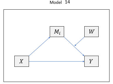

동일한 자료로 분석한 결과
Model 14 : M --> Y 의 조절효과 유의함
Model 15 : M --> Y 의 조절효과 유의하지 않음
분석 결과를 보면 조절된 매개효과 역시
*****************************************
Model 14
Index of moderated mediation:
Index BootSE BootLLCI BootULCI
scom_avg -.1026 .0223 -.1471 -.0590
*****************************************
Model 15
Index of moderated mediation:
Index BootSE BootLLCI BootULCI
scom_avg -.0528 .0344 -.1158 .0187
*****************************************
Model 14 에서는 조절된 매개효과가 유의하게 나오는 반면 Model 15 에서는 조절된 매개효과가 유의하지 않게 나옵니다.
일단 Model 14, 15 로 분석한 경우 그 결과가 지금처럼 서로 상이하게 나오는 경우는 흔한 일입니다.
Model 1, 4 에서 유의했다고 해서 그 결과가 Model 14, 15 까지 유지되지 않습니다.
오히려 반대의 결과가 나오는 경우도 흔한 일입니다.
분석 결과를 보면
X --> M --> Y
의 간접효과는 Model 14, 15 모두 유의하게 나옵니다.
그런데, 이 간 접효과가 조절변수에 따라 달라지는지 확인해 보면
Model 15 에서는 간접효과가 조절변수에 영향을 받지 않은데 비하여
Model 14 에서는 조절변수가 커질수록 X --> M --> Y 의 양(+)의 간접효과가 작아지는 것을 확인할 수 있습니다.
대신 Model 15 에서는 X --> Y 에 미치는 직접효과가 조절변수에 따라 달라지는 것으로 나옵니다.
조절변수가 커질수록 X --> Y 에 미치는 양(+)의 직접효과가 작아지는 것으로 나옵니다.
Model 14, 15 중에서 어느 모형을 선택할지는 결국 연구자의 선택입니다.
이상의 결과를 정리한다면 저 같으면 Model 15 로 설정하겠습니다.
X -> Y 에 유의한 직접효과를 준단
X -> Y 의 직접효과를 조절변수가 조절한다.
X -> M -> Y 의 간접효과가 유의하다
고급 통계분석의 관점에서 본다면 조절된 매개효과가 더 있어보이지만, 모형을 설명한다는 측면에서는 Model 15 도 충분한 메리트가 있는 해석이 나옵니다.
석따 (2024-11-16 22:04:22)
교수님, 좋은 말씀 감사합니다.
Legacy document_srl: 304736 / Legacy URL: http://www.statedu.com/QnA/304736
댓글